Stereo Reconstruction from Scratch

Theory

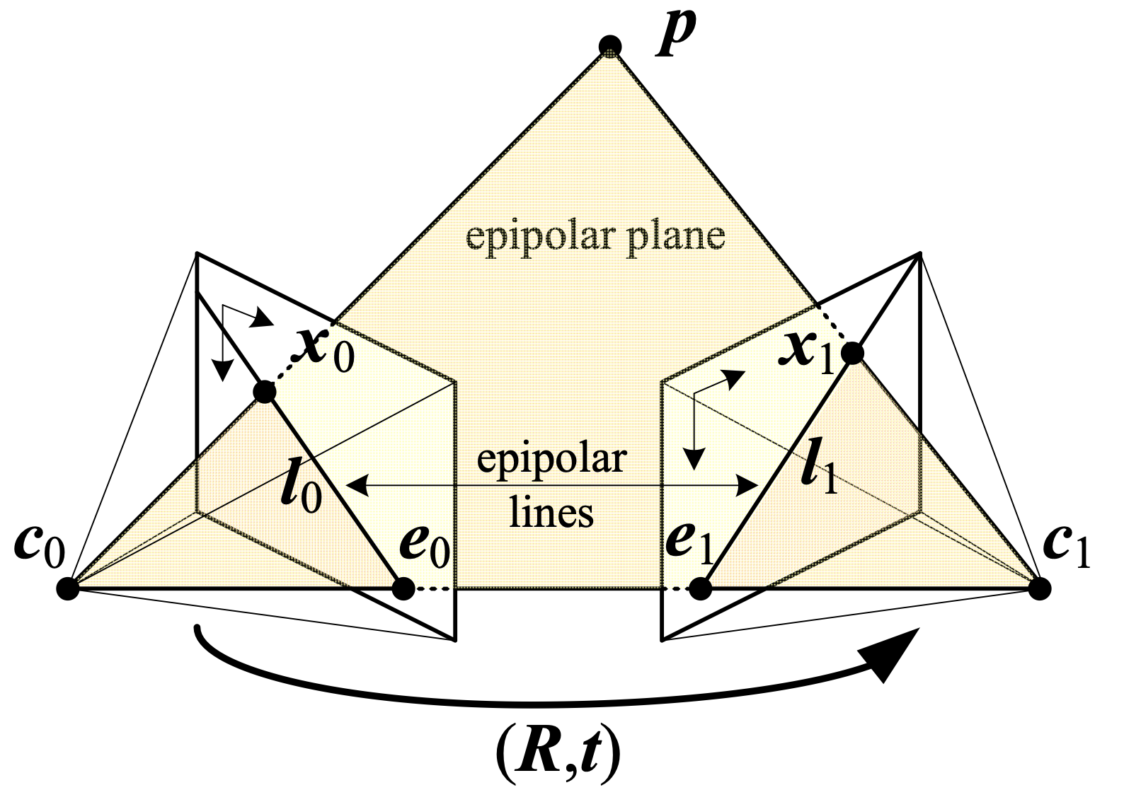
Stereo matching is the process of taking two images and constructing a 3D model of the scene by identifying corresponding pixels in both images. The objective is to convert 2D pixel positions into 3D depth information

[1] . The theoretical foundation of stereo matching is epipolar geometry. Let's take a look at the following figure.

c_0 and c_1 are the centers of the left and right cameras for a given stereo setup. The baseline is the line connecting c_0 and c_1 . A real-world 3D point p projects onto the image planes as points x_0 and x_1 . The key geometric constraint is that the three points c_0 , p , and c_1 define a plane called the epipolar plane. Each epipolar plane intersects the image planes along lines called epipolar lines, denoted as l_0 and l_1

[2] . This implies that given a point x_0 in the left image, its corresponding point x_1 in the right image must lie on the corresponding epipolar line l_1

"Multiple view geometry in computer vision"
Richard Hartley and Andrew Zisserman, 2003

[2] . This constraint significantly reduces the search space for matching points from the whole 2D image plane, down to a single line.
Although epipolar geometry applies to any roto-translation between c_0 and c_1 , images are often rectified in practice

"Computer vision: algorithms and applications"
Richard Szeliski, 2022

[1] . Rectification involves warping the input images so that corresponding horizontal scanlines become epipolar lines

"Computer vision: algorithms and applications"
Richard Szeliski, 2022

[1] . This transformation results in the following relationship between the pixel coordinates x_0 = (u_0, v_0) and x_1 = (u_1, v_1)

u_1 = u_0 + d(u_0,v_0) \qquad v_1 =v_0

where d(u_0,v_0) is called the disparity at pixel location x_0 . This means that corresponding points can be found along the same horizontal line, by simply adding an offset. Collecting the disparities for all image locations produces the disparity map. For the purposes of this project, it is always assumed that the input images are rectified. Once the disparity d(u_0,v_0) is known, the following projection equation can be rearranged to obtain the depth Z of the point p

d(u_0,v_0) = f \frac{B}{Z}

Here f is the focal length (a property of the camera) and B is the baseline (the distance between the two cameras). The main question is now, how can d(u_0,v_0) be computed?

As the image capturing process is inherently affected by noise, the exact disparity cannot be computed. Therefore, the disparity needs to be estimated. Various approaches exist for estimating the disparity. Discussing all of them is beyond the scope of this blog post. We focus on two popular groups of approaches:

• Local methods: These methods aggregate the matching cost by summing or averaging over a support region
  "Computer vision: algorithms and applications"
  Richard Szeliski, 2022
  [1] . A cost function C(u, v, d) is computed over this region, and the estimated disparity d^* is then the disparity that minimizes the cost d^* = \underset{d}{\text{argmin}} ~ C(u, v, d)
• Global methods: These methods are formulated within an energy-minimization framework, where the objective is to find a disparity function d that minimizes a global energy E(d) = E_D(d) + \lambda E_S(d) where E_D(d) measures how well the disparity function agrees with the input image pair, and E_S(d) enforces smoothness constraints, i.e., that neighboring pixels should have similar disparity values
  "Computer vision: algorithms and applications"
  Richard Szeliski, 2022
  [1] . Performing this energy minimization in the 2D plane is known to be NP-hard
  "Computer vision: algorithms and applications"
  Richard Szeliski, 2022
  [1] . However, for the 1D case, efficient algorithms exist to solve the energy-minimization problem
  "Fast approximate energy minimization via graph cuts"
  Yuri Boykov, Olga Veksler, and Ramin Zabih, 2002
  [3] . Combining multiple 1D optimization directions and aggregating their path costs leads to semi-global matching methods
  "Stereo processing by semiglobal matching and mutual information"
  Heiko Hirschmuller, 2007
  [4] . Semi-global matching algorithms are both efficient and perform well in practice
  "Computer vision: algorithms and applications"
  Richard Szeliski, 2022
  [1] .

In the next section, one implementation from each group is described in detail.

Block Matching Implementation

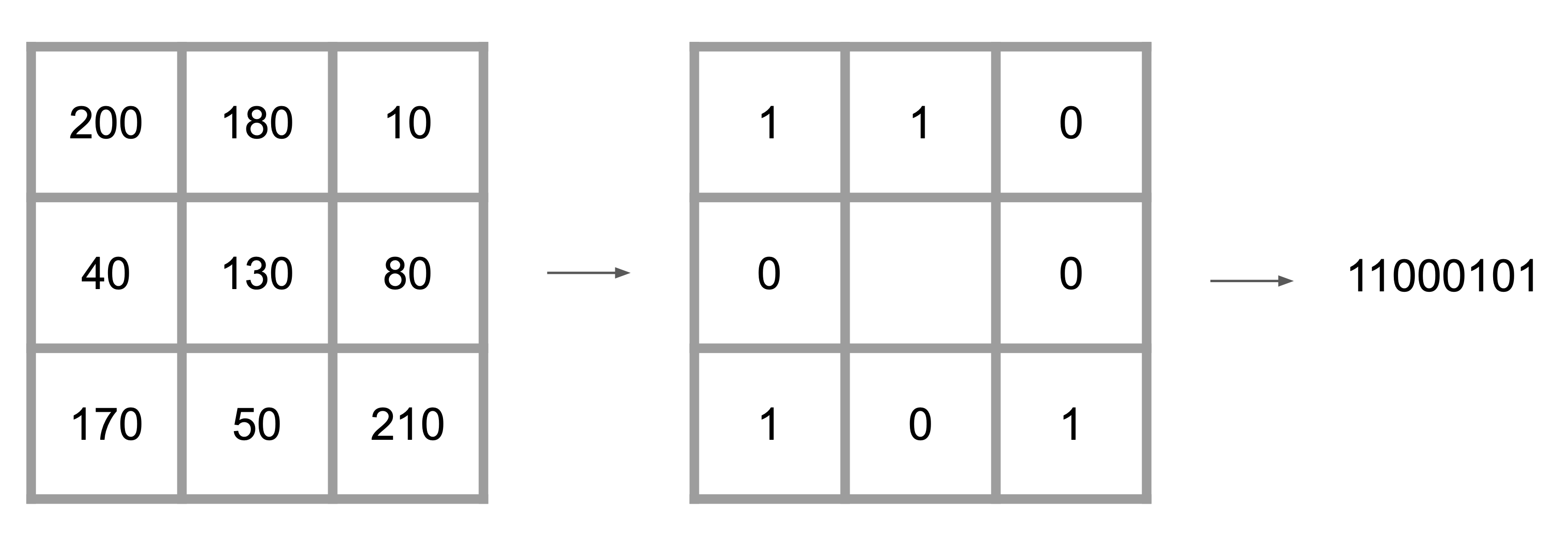
Block matching is one of the simplest local stereo matching approaches. In this project, block matching is implemented by moving a window along the corresponding horizontal line in the right image I_1 for every pixel (u,v) in the left image I_0 . For every offset d \in { \{0,\dots,D \}} , the cost C(u,v,d) is computed, where D is the fixed maximum disparity. In the implementation, the mean squared error is used as the matching cost function

C(u,v,d) = \frac{1}{N} \sum_{(i,j) \in R} {[}I_0(u+i,v+j) - I_1(u+i-d,v+j){]^2}

The estimated disparity d^* is then the disparity with the lowest cost

d^* = \underset{d}{\text{argmin}} ~ C(u, v, d)

In the project implementation, a window size of 15 and a maximum disparity D of 64 were used. Note that the offset is subtracted from the image coordinates. Following the projection rules for rectified images, the image coordinates of a point in the right image are farther left than the coordinates of the same point in the left image. This algorithm can directly be implemented in Python. Here is a simplified version of my implementation.

class BM:
    
    def __init__(self):
        self.kernel_size = 15
        self.max_disparity = 64
        self.kernel_half = 7
        # offset_adjust is used to map depth map output to 0-255 range
        self.offset_adjust = 255 / self.max_disparity  
        
    def _get_window(self, y, x, img, offset=0):
        """Get the window centered at (y, x) with the given offset"""
        y_start = y-self.kernel_half
        y_end = y+self.kernel_half
        x_start = x-self.kernel_half-offset+1
        x_end = x+self.kernel_half-offset+1
        return img[y_start:y_end,x_start:x_end]
    
    def compute(self, left, right):
        h, w = left.shape
        disp_map = np.zeros_like(left, dtype=np.float32)
        for y in range(self.kernel_half, h - self.kernel_half):      
            for x in range(self.max_disparity, w - self.kernel_half):
                best_offset = None
                min_error = float("inf")
                errors = []
                for offset in range(self.max_disparity):               
                    W_left = self._get_window(y, x, left)
                    W_right = self._get_window(y, x, right, offset)
                    if W_left.shape != W_right.shape:
                        errors.append(None)
                        continue
                    error = np.sum((W_left - W_right)**2)
                    errors.append(np.float32(error))
                    if error < min_error:
                        min_error = error
                        best_offset = offset
                disp_map[y, x] = best_offset * self.offset_adjust
        return disp_map

The important stuff happens in the compute method. At the beginning, the disparity map is initialized to zeros. Then, for every pixel in the left image, a window is extracted from the left image and the right image. The window is centered at the pixel location (y,x) in the left image and at (y,x-offset) in the right image. The offset is varied from 0 to max_disparity. The sum of squared differences between the two windows is computed and stored in a list. The offset with the lowest cost is then assigned to the disparity map. The final disparity map is scaled to fit into the range of 0-255.

Semi-Global Matching Implementation

The Semi-Global Matching (SGM) algorithm presented by Hirschmüller

[4] is based on the idea of pixel-wise matching and approximating a global 2D smoothness constraint by combining many 1D constraints

"Stereo processing by semiglobal matching and mutual information"
Heiko Hirschmuller, 2007

[4] . The implementation of the Semi-Global Matching algorithm in this project is inspired by

"Stereo processing by semiglobal matching and mutual information"
Heiko Hirschmuller, 2007

[4] , but it is not identical. Some of the resources I used for my implementation that may be helpful for understanding the algorithm are

"Semi-global matching"
Wikipedia, 2025 (Accessed 28.04.2025)

[5] ,

"Semi-Global Matching Numpy"
Christian Orr, 2025 (Accessed 28.04.2025)

[6] ,

"Semi-Global Matching"
David-Alexandre Beaupre, 2025 (Accessed 28.04.2025)

[7] and

"Reddit"
Tr0xyzz1s, 2025 (Accessed 28.04.2025)

[8] . The distinct processing steps of the implementation are discussed in the following paragraphs.

Instead of matching pixels by their grayscale values, the census transform

[9] is applied to the left and right images. The census transform computes a bit string for each pixel, which is then used for matching. The census transform generates a bit string based on the relative intensities of the neighboring pixels. If the intensity of a neighboring pixel is less than that of the center pixel, a 1 is added to the bit string; otherwise, a 0 is added. This operation is repeated for all neighboring pixels to create the bit string. The ordering of the bits in the string contains enough information to perform an accurate and fast correspondence operation. The census transform computation is implemented by iterating over the image and calculating the census transform for each pixel. The bit string is stored as an integer.

After applying the census transform to the left and right images, the Hamming distance is used to compute the cost. The Hamming distance compares two bit strings and counts the number of differing bits (e.g., 101 and 110 have a Hamming distance of 2 since they differ in two bits). The computation of the cost C(u,v,d) for the pixel (u,v) and disparity d \in \{1, \dots, D \} can be implemented as follows

C(u, v, d) = CT_0 (u,v) \oplus CT_1 (u-d,v)

Here, \oplus denotes the logical XOR operation, CT_0 and CT_1 are the census-transformed images, and the summation is performed over the bit string. The cost computation step can be implemented by iterating over d \in \{1, \dots, D \} , shifting the right image CT_1 by d pixels, and computing C(u, v, d) pixel-wise. The NumPy library can be leveraged to perform this computation efficiently. All costs are collected in a cost volume with dimensions \mathbb{N}^{H \times W \times D} , where H and W are the image dimensions, and D is the maximal disparity.

Pixelwise cost calculation is generally ambiguous and noisy. As mentioned in the theory section, minimizing the energy in 2D is NP-hard

[1] . Therefore, Hirschmüller proposes to minimize the energy in 1D for different directions r and aggregate the costs. This acts as an additional constraint that supports smoothness by penalizing changes in neighboring disparities

"Stereo processing by semiglobal matching and mutual information"
Heiko Hirschmuller, 2007

[4] . This results in a smoother cost volume and hence a smoother disparity map. The path cost L_r (p, d) for a pixel p and direction r is computed by the following expression

L_r (p, d) = C(p,d) - \underset{k}\min ~ L_r(p-r,k) + \min\begin{cases} L_r(p-r,d) \\ L_r(p-r, d-1) + P_1 \\ L_r(p-r, d+1) + P_1 \\ \underset{i}{\min} ~ L_r(p-r,i) + P_2 \end{cases}

The second term is used to prevent L_r(p,d) from permanently increasing along the path

[4] . P_1 and P_2 are constant penalties, where P_1 penalizes small disparity changes and P_2 penalizes larger disparity changes

"Stereo processing by semiglobal matching and mutual information"
Heiko Hirschmuller, 2007

[4] . Using a lower penalty for small changes permits adaptation to slanted or curved surfaces

"Stereo processing by semiglobal matching and mutual information"
Heiko Hirschmuller, 2007

[4] . In the project implementation, the penalties are set to P_1 = 10 and P_2 = 120 . The costs L_r are summed over paths in all directions r to obtain the aggregated (smoothed) cost

S(p,d) = \sum_r L_r(p,d)

Although Hirschmüller recommends using 8 to 16 paths

[4] , Žbontar and LeCun state that they gained no accuracy improvement from using more than 4 paths

"Stereo Matching by Training a Convolutional Neural Network to Compare Image Patches"
Jure Žbontar and Yann LeCun, 2015

[10] . Therefore, the SGM algorithm implemented in this project uses 4 paths (i.e., north, south, east, west directions). Note that the smoothed costs form a cost volume S \in \mathbb{N}^{H \times W \times D} . By selecting

d^* = \underset{d}{\text{argmin}} ~ S(p,d)

for every pixel p , the final disparity map can be extracted from the cost volume. Now let's take a look at the code. The code for computing the census transform is straightforward

def census_transform(self, img):
    height, width = img.shape
    census_values = np.zeros_like(img, dtype=np.int32)
    for y in range(self.kernel_half, height - self.kernel_half):
        for x in range(self.kernel_half, width - self.kernel_half):
            patch = self._get_patch(y, x, img)
            # If value is less than center value assign 1 otherwise assign 0 
            census_pixel_array = (patch.flatten() > img[y, x]).astype(int)
            # Convert census array to an integer by using bit shift operator
            census_values[y, x] = np.int32(census_pixel_array.dot(1 << np.arange(self.kernel_size * self.kernel_size)[::-1])) 
    return census_values

Here, the _get_patch method extracts the patch around the pixel (y,x). Next, the transformed images are used to compute the matching cost using the Hamming distance

def compute_costs(self, left_census_values, right_census_values):
    height, width = left_census_values.shape
    cost_volume = np.zeros(shape=(height, width, self.max_disparity), dtype=np.uint32)
    census_tmp = np.zeros_like(left_census_values, dtype=np.int32)

    for d in range(self.max_disparity):
        # The right image is shifted d pixels accross
        census_tmp[:, self.kernel_half+d:width-self.kernel_half] = right_census_values[:, self.kernel_half:width-d-self.kernel_half]
        # 1 is assigned when the bits differ and 0 when they are the same
        xor = np.bitwise_xor(left_census_values, census_tmp)
        # All the 1's are summed up to give us the number of different pixels (the cost)
        distance = np.bitwise_count(xor)
        # All the costs for that disparity are added to the cost volume
        cost_volume[:, :, d] = distance
    return cost_volume

First, the cost volume and the temporary census image are initialized. Then, for each disparity d, the right image is shifted d pixels to the left. The Hamming distance is computed by applying the XOR operation to the two census images. The number of differing bits is then summed up and stored in the cost volume.

def _get_path_cost(self, slice, offset, penalties, other_dim):
    """Compute the minimum cost path for a single direction"""
    minimum_cost_path = np.zeros(shape=(other_dim, self.max_disparity), dtype=np.int32)
    minimum_cost_path[offset - 1, :] = slice[offset - 1, :]

    for pixel_index in range(offset, other_dim):
        # Get all the minimum disparities costs from the previous pixel in the path
        previous_cost = minimum_cost_path[pixel_index - 1, :]
        # Get all the disparities costs (from the cost volume) for the current pixel
        current_cost = slice[pixel_index, :]
        costs = np.repeat(previous_cost, repeats=self.max_disparity, axis=0).reshape(self.max_disparity, self.max_disparity)
        # Add penalties to the previous pixels disparities that differ from current pixels disparities
        costs = costs + penalties
        # Find minimum costs for the current pixels disparities using the previous disparities costs + penalties 
        costs = np.amin(costs, axis=0)  
        # Current pixels disparities costs + minimum previous pixel disparities costs (with penalty) - 
        # (constant term) minimum previous cost from all disparities 
        pixel_direction_costs = current_cost + costs - np.amin(previous_cost)
        minimum_cost_path[pixel_index, :] = pixel_direction_costs

    return minimum_cost_path 

def _aggregate_costs(self, cost_volume):
    """Aggregate costs in all directions"""
    height, width, _ = cost_volume.shape
    p2 = np.full(shape=(self.max_disparity, self.max_disparity), fill_value=self.penalty2, dtype=np.int32)
    p1 = np.full(shape=(self.max_disparity, self.max_disparity), fill_value=self.penalty1 - self.penalty2, dtype=np.int32)
    p1 = np.tril(p1, k=1) 
    p1 = np.triu(p1, k=-1)
    no_penalty = np.identity(self.max_disparity, dtype=np.int32) * -self.penalty1
    penalties = p1 + p2 + no_penalty

    south_aggregation = np.zeros(shape=(height, width, self.max_disparity), dtype=np.float32)
    north_aggregation = np.copy(south_aggregation)

    for x in range(self.kernel_half, width-self.kernel_half):
        # Takes all the rows and disparities for a single column
        south = cost_volume[:, x, :]
        # Invert the rows to get the opposite direction
        north = np.flip(south, axis=0)
        south_aggregation[:, x, :] = self._get_path_cost(south, 1, penalties, height)
        north_aggregation[:, x, :] = np.flip(self._get_path_cost(north, 1, penalties, height), axis=0)

    east_aggregation = np.copy(south_aggregation)
    west_aggregation = np.copy(south_aggregation)
    for y in range(self.kernel_half, height-self.kernel_half):
        # Takes all the column and disparities for a single row
        east = cost_volume[y, :, :]
        # Invert the columns to get the opposite direction
        west = np.flip(east, axis=0)
        east_aggregation[y, :, :] = self._get_path_cost(east, 1, penalties, width)
        west_aggregation[y, :, :] = np.flip(self._get_path_cost(west, 1, penalties, width), axis=0)

    # Combine the costs from all paths into a single aggregation volume
    aggregation_volume = np.concatenate((south_aggregation[..., None], north_aggregation[..., None], east_aggregation[..., None], west_aggregation[..., None]), axis=3)
    return aggregation_volume

The _aggregate_costs method takes this cost volume and initializes the penalties. Next, two additional volumes are created to store the aggregated costs for the south and north directions. The _get_path_cost method is called for every pixel in the column. The same is done for the east and west directions. Finally, all four volumes are concatenated to form the final cost volume.

def _select_disparity(self, aggregation_volume):
    # sum up costs for all directions
    volume = np.sum(aggregation_volume, axis=3).astype(float)
    # returns the disparity index with the minimum cost associated with each h x w pixel
    disparity = np.argmin(volume, axis=2).astype(float)
    return disparity

Finally, the aggregated costs are summed up and the disparity with the lowest cost is selected.

def compute(self, left, right):
    left_census = self._census_transform(left)
    right_census = self._census_transform(right)
    cost_volume = self._compute_costs(left_census, right_census)
    aggregation_volume = self._aggregate_costs(cost_volume)
    disparity = self._select_disparity(aggregation_volume)
    return disparity

All pieces are put together in the compute method. In the implementation on GitHub additional scaling of the disparity between 0 and 255 is applied for visualization purposes. Here, the scaling is omitted for simplicity.

Sub-Pixel Estimation

So far, all algorithms compute a discrete disparity value d \in \{ 1 \dots D \}

[1] . When reconstructing the point cloud from the disparity map, this results in discrete levels of the disparity map. Since this does not correspond to a realistic reconstruction of the scene, sub-pixel estimation can be used to obtain a more continuous scene reconstruction. Sub-pixel estimation uses the costs of the two neighboring disparities C(d^*-1) and C(d^*+1) of the optimal disparity d^* to compute the minimum of the parabola interpolated through the three points.

d^*_{\text{ref}} = d^* + \frac{C(d^*-1) - C(d^*+1)}{2C(d^*-1) - 4C(d^*) + 2C(d^*+1)}

The refined disparity d^*_{\text{ref}} is then stored in the final disparity map. In the project implementation, sub-pixel estimation can be activated for both algorithms with a command-line argument.

Results

Now it's time to take a look at the results. The implemented algorithms have been evaluated on two selected scenes from the Middlebury stereo dataset collection

[11] ,

"Learning conditional random fields for stereo"
Daniel Scharstein and Chris Pal, 2007

[12] ,

"Evaluation of cost functions for stereo matching"
Heiko Hirschmuller and Daniel Scharstein, 2007

[13] . All images have dimensions of 450 \times 375 pixels. The following image shows the computed disparity maps of the implemented methods without sub-pixel estimation. The OpenCV disparity map is included for reference.

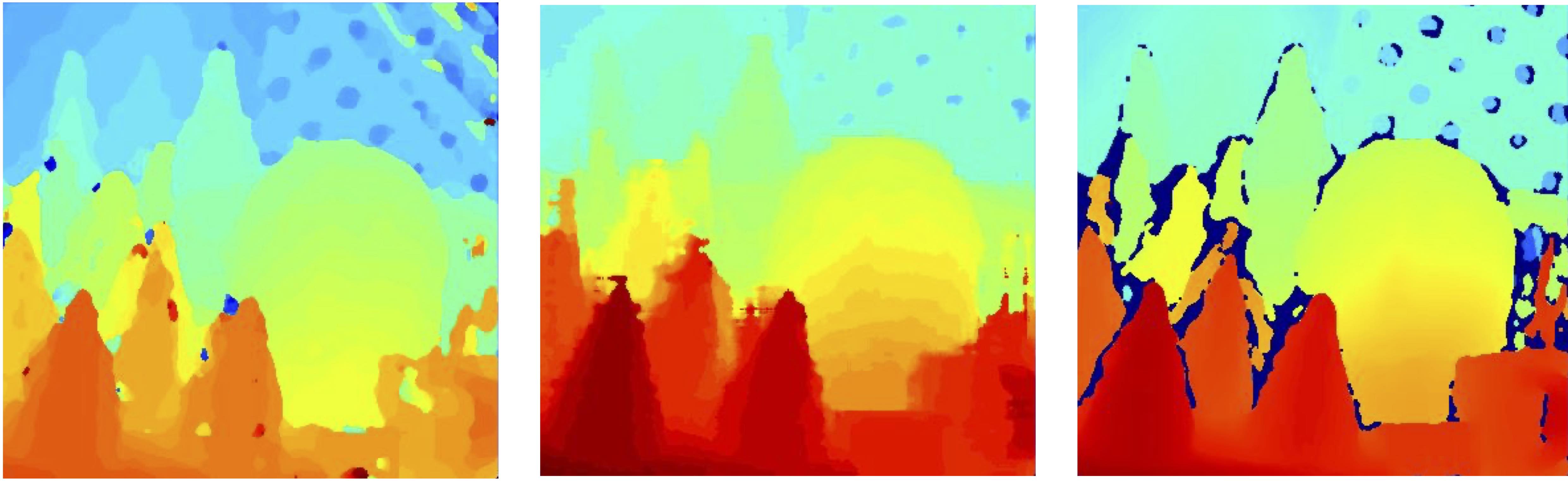
The SGM algorithm produces a smoother disparity map, with fewer holes (deep blue patches in the disparity map). However, the smoothing in the SGM algorithm also removes some details in the background (e.g., in the top right corner). The OpenCV algorithm performs an additional left-right consistency check by computing disparity maps for both the left and right images. This allows the OpenCV algorithm to mark occluded pixels as invalid (i.e., assigning them a disparity of zero). Both implemented algorithms do not use a left-right consistency check, and therefore, occluded pixels are assigned a disparity. The following image demonstrates that the activation of sub-pixel estimation produces a smoother disparity map

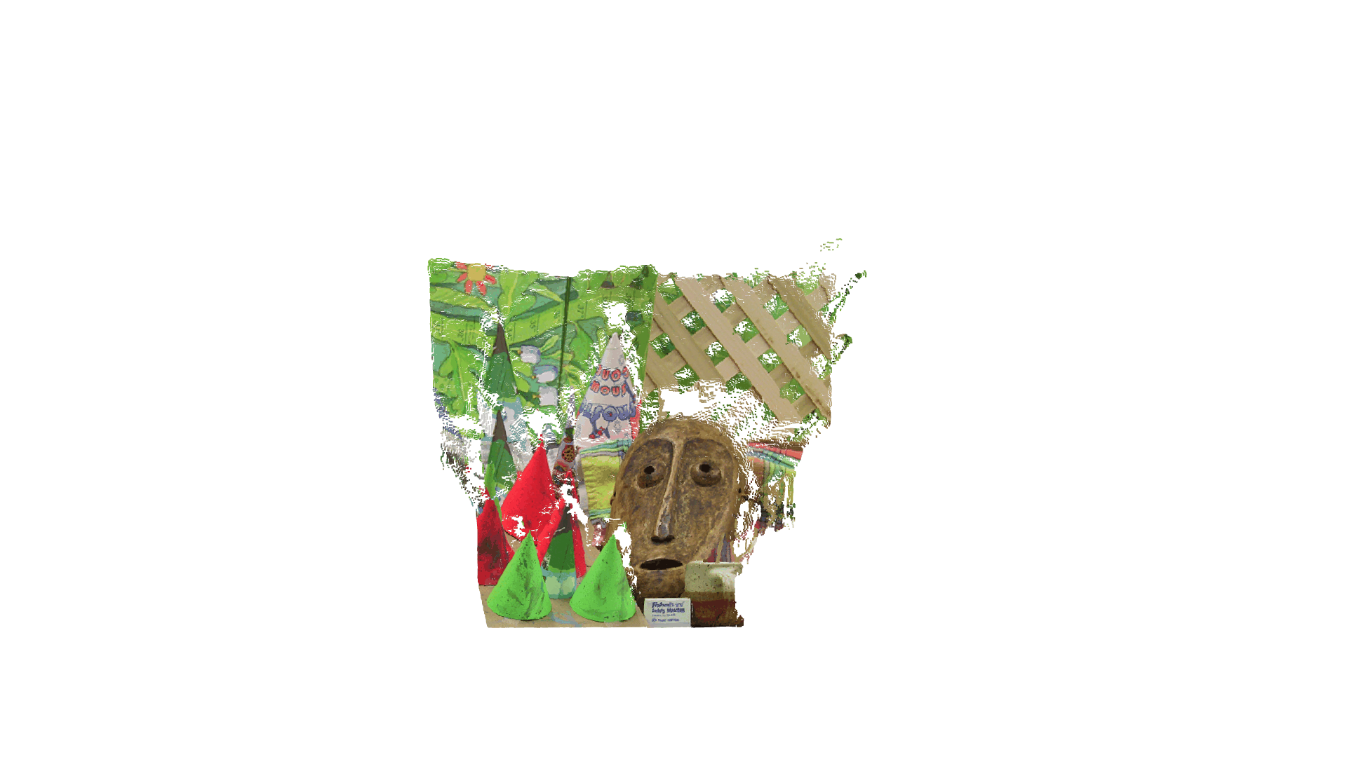
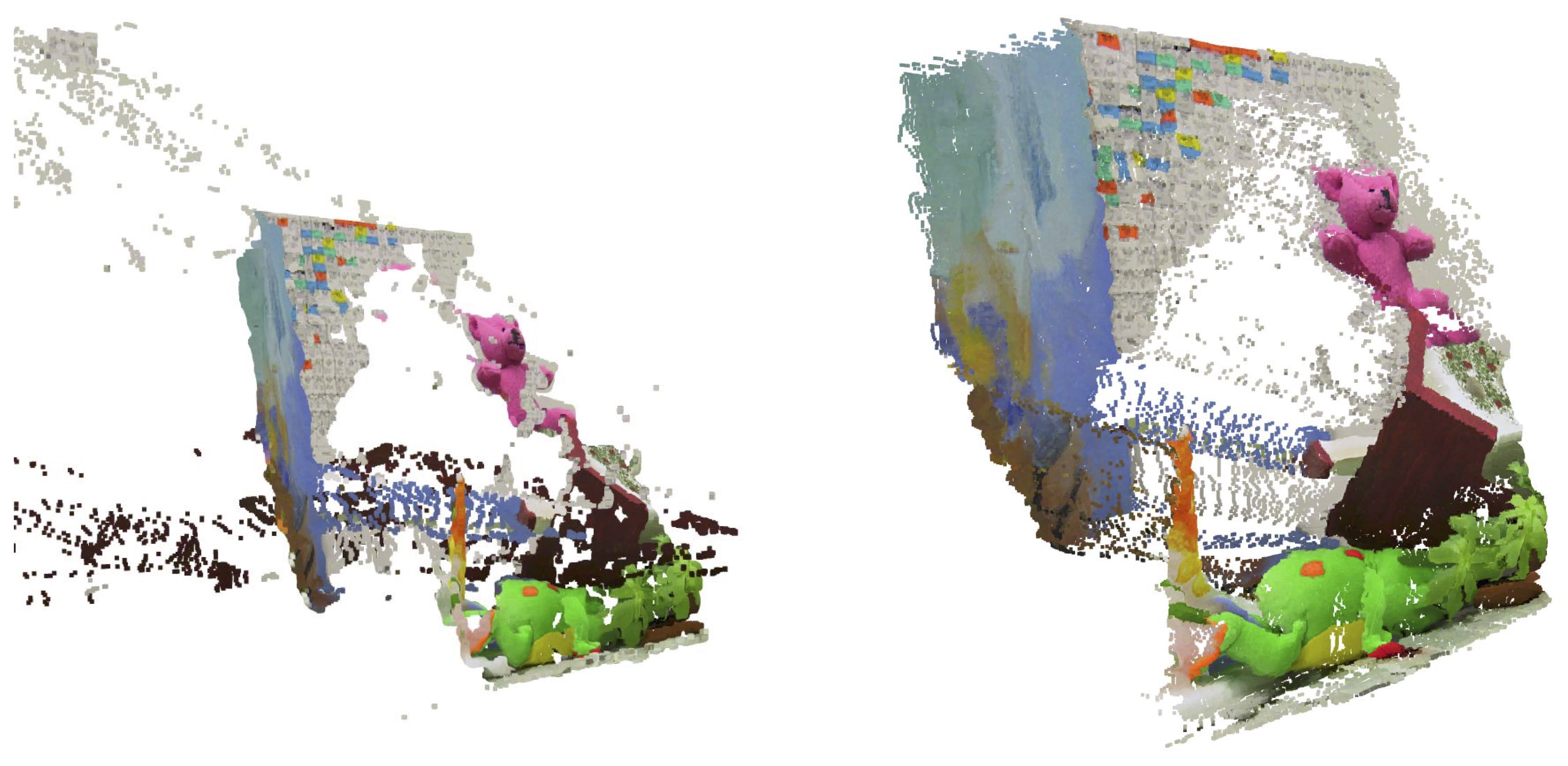
The effects of sub-pixel estimation on the reconstructed point cloud can be observed in the following image

Especially for the mask and the rounded cones, sub-pixel estimation produces more realistic reconstructions of the scene compared to disparity maps without sub-pixel estimation. Apart from a qualitative evaluation, quantitative metrics can be computed as the Middlebury stereo datasets provide ground truths

[11] ,

"Learning conditional random fields for stereo"
Daniel Scharstein and Chris Pal, 2007

[12] ,

"Evaluation of cost functions for stereo matching"
Heiko Hirschmuller and Daniel Scharstein, 2007

[13] . The percentage of bad pixels (PBP) for different algorithms and images is reported. PBP reports the percentage of pixels where the difference between estimated and true disparity is greater than a given threshold \tau

\text{PBP} = \frac{\sum_{i} \mathbb{I} \left( |d_i - d^*_i| > \tau \right)}{H \times W} \times 100

The next table reports the PBP for the selected scences and the implemented algorithms. The threshold \tau is set to 3 pixels.

According to this table, block matching with sub-pixel estimation produces the best results on the two tested image pairs. Nonetheless, it is important to note that the evaluation of the different algorithms during this project is by far not exhaustive. A larger dataset and a more systematic evaluation of the disparity map quality are needed to make justified claims about the algorithm's performance. Overall, the generated point clouds appear to be a reasonable reconstruction of the scene. Visually, the SGM algorithm with sub-pixel estimation seems to produce the best results with only a few outliers.

Future Work

Future work can be pursued in various directions. Additional algorithms could be implemented, and neural network approaches could be integrated into the project. A broader benchmarking of the algorithm's performance would be beneficial, especially for challenging scenes. Furthermore, optimizations such as left-right consistency checks could be implemented to improve the handling of occluded image regions. Lastly, further improvements in processing time could be achieved by leveraging different hardware capabilities such as vectorization or GPU computing. On the software side, optimizations such as computing the integral image for cost computation could lead to improved processing times.

References

[1] Richard Szeliski. "Computer vision: algorithms and applications", 2022

[2] Richard Hartley and Andrew Zisserman. "Multiple view geometry in computer vision", 2003

[3] Yuri Boykov, Olga Veksler, and Ramin Zabih. "Fast approximate energy minimization via graph cuts", 2002

[4] Heiko Hirschmuller. "Stereo processing by semiglobal matching and mutual information", 2007

[5] Wikipedia. "Semi-global matching", 2025 (Accessed 28.04.2025)

[6] Christian Orr. "Semi-Global Matching Numpy", 2025 (Accessed 28.04.2025)

[7] David-Alexandre Beaupre. "Semi-Global Matching", 2025 (Accessed 28.04.2025)

[8] Tr0xyzz1s. "Reddit", 2025 (Accessed 28.04.2025)

[9] Ramin Zabih and John Woodfill. "Non-parametric local transforms for computing visual correspondence", 1994

[10] Jure Žbontar and Yann LeCun. "Stereo Matching by Training a Convolutional Neural Network to Compare Image Patches", 2015

[11] Daniel Scharstein and Richard Szeliski. "High-accuracy stereo depth maps using structured light", 2003

[12] Daniel Scharstein and Chris Pal. "Learning conditional random fields for stereo", 2007

[13] Heiko Hirschmuller and Daniel Scharstein. "Evaluation of cost functions for stereo matching", 2007